
Introduction to Neural Networks
Overview
- Introduction
- Neural Networks Basics
- Data Preprocessing
- Backpropagation
- Optimization
- Stability, Learning Dynamics and Hyperparameters
- Evaluation Methodology
- Model Fit and Regularization
Introduction
Applications of Neural Networks
Why Neural Networks?
- Traditional ML limitations:
- Manual feature engineering required
- Difficulty with complex patterns
- Poor scalability with high-dimensional data
- Neural Network advantages:
- Automatic feature learning
- Superior performance on complex tasks
- Ability to handle multiple data types
- Transfer learning capabilities
What are Neural Networks?
- A computational model inspired by biological neural networks.
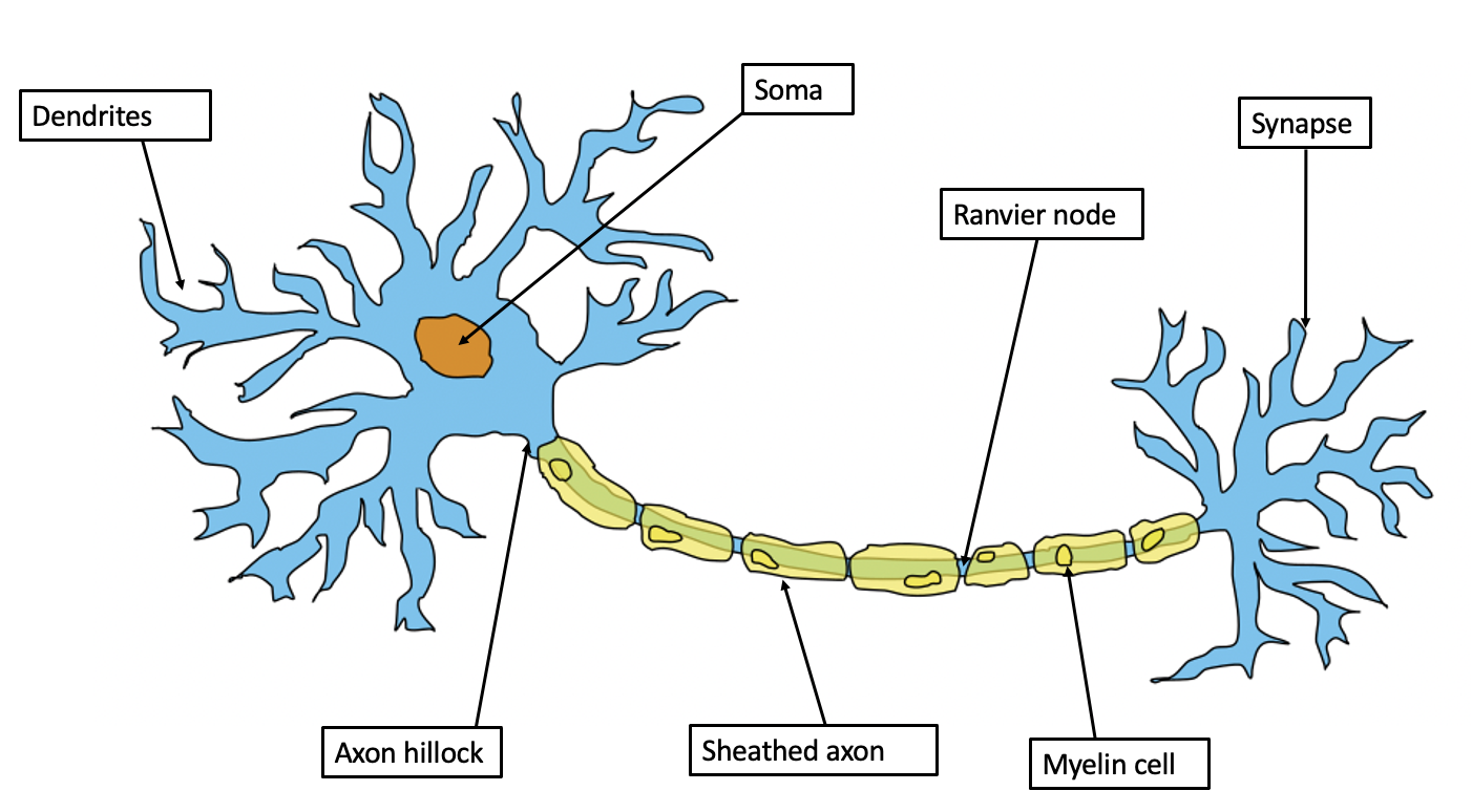
- Composed of layers of interconnected nodes (neurons).
- Can model complex patterns and relationships in data.
Common Misconceptions
- "Neural networks work like the human brain"
- Reality: Only loosely inspired by biological neurons
- Major differences in structure and learning process
- "More layers always mean better performance"
- Reality: Deeper isn't always better
- Architecture should match problem complexity
- "Neural networks are a black box"
- Reality: Various interpretation techniques exist
- Gradients and activations can be analyzed
- "Neural networks need massive datasets"
- Reality: Transfer learning enables use with smaller datasets
- Data efficiency techniques exist
Brief History
Our Objective
- Understand the foundational concepts of neural networks.
- Learn how they process and classify data.
Neural Network Basics
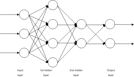
Structure of a Neural Network
- Composed of layers:
- Input layer: Receives input features
- Hidden layers: Extract patterns and features
- Output layer: Produces predictions
- Each layer contains interconnected nodes (neurons)
- Weights and biases determine the importance of connections
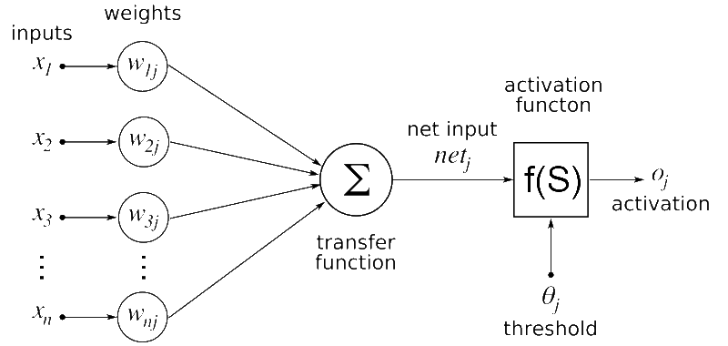
Forward Pass
- Data flows sequentially through the network:
- Inputs are multiplied by weights and added to biases
- An activation function introduces non-linearity
- Each layer's output becomes the input for the next layer
Activation Functions
- Add non-linearity to the network
- Enable learning of complex patterns
- Transform neuron outputs into useful ranges
Common Activation Functions
- ReLU:
- \( f(x) = \max(0, x) \)

- Most widely used in hidden layers
- Cheap to compute; mitigates vanishing gradients
- \( f(x) = \max(0, x) \)
- Leaky ReLU:
- \( f(x) = \max(0.01x, x) \)

- Small gradient for negative inputs
- Reduces risk of “dead” ReLU neurons
- \( f(x) = \max(0.01x, x) \)
- Sigmoid:
- \( \sigma(x) = \frac{1}{1 + e^{-x}} \)

- Output in (0, 1)
- Used in binary classification output layers
- \( \sigma(x) = \frac{1}{1 + e^{-x}} \)
- Tanh:
- \( \tanh(x) = \frac{e^x - e^{-x}}{e^x + e^{-x}} \)

- Output in (−1, 1), zero-centered
- Historically common in recurrent networks
- \( \tanh(x) = \frac{e^x - e^{-x}}{e^x + e^{-x}} \)
- Softmax (output layer):
- \( \hat{y}_i = \frac{e^{z_i}}{\sum_j e^{z_j}} \)
- Used in multiclass output layers
- Converts logits into a probability distribution
- \( \hat{y}_i = \frac{e^{z_i}}{\sum_j e^{z_j}} \)
Loss Functions
- Role:
- Quantifies the error between predicted (\( \hat{y} \)) and true values (\( y \))
- Guides weight and bias adjustments through optimization
- Essential for training the neural network
- Where it fits:
- Occurs after the forward pass
- Calculates the error, which is used in backpropagation
- Optimizers (e.g., gradient descent) minimize the loss
Loss Functions (continued)
- Mean Squared Error (MSE):
- \( L = \frac{1}{n}\sum (y - \hat{y})^2 \)
- Used for regression problems
- Sensitive to outliers
- Binary Cross-Entropy:
- \( L = -(y \log(\hat{y}) + (1 - y) \log(1 - \hat{y})) \)
- Used for binary classification problems
- Penalizes confident wrong predictions
- Multiclass Softmax + Cross-Entropy:
- Softmax mapping: \( \hat{y}_i = \text{softmax}(z)_i = \frac{e^{z_i}}{\sum_j e^{z_j}} \)
- Loss: \( L = -\sum_{i=1}^K y_i \log(\hat{y}_i) \)
- Used for multiclass classification with one-hot or probabilistic targets
- Penalizes confident wrong assignments; with softmax, invariant to additive shifts in logits
Neural Network Architectures
| Architecture | Data Adapted | Use Cases |
|---|---|---|
| Feedforward Networks (FFN) | Structured, tabular data | Regression, simple classification tasks |
| Convolutional Neural Networks (CNN) | Grid-like data (e.g., images) | Image recognition, object detection, spatial pattern recognition |
| Recurrent Neural Networks (RNN) | Sequential data (e.g., time series, text) | Natural Language Processing (NLP), time series forecasting |
| Transformers | Long sequences, complex relationships | Language modeling, translation, long-range dependencies |
Neural Network Architectures (continued)
Transformer Architecture
- Core Components:
- Self-attention mechanism
- Multi-head attention
- Position encodings
- Feed-forward networks
- Key Benefits:
- Captures long-range dependencies
- Enables parallel computation
- Reduces—but does not eliminate—gradient degradation issues compared to RNNs
- Applications:
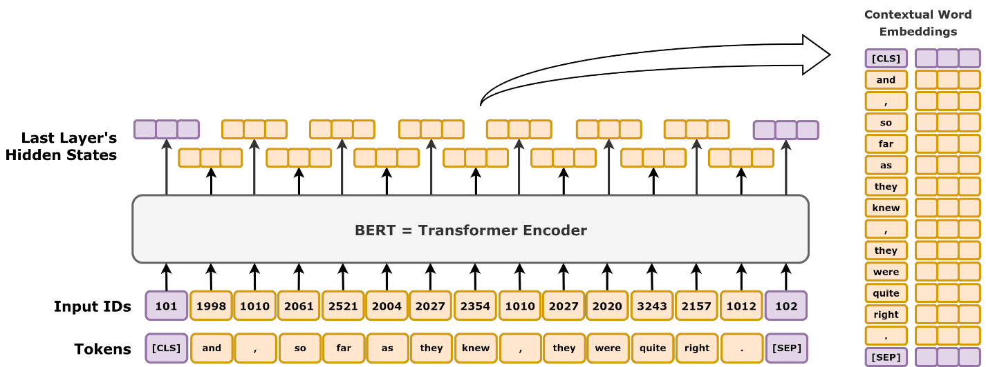
- Language models (GPT, BERT)
- Machine translation
- Vision tasks (ViT)
Data Preprocessing
Data Preprocessing
Essential first step for neural network training
- Ensures consistent scale across features
- Speeds up training
- Improves model stability
Common techniques
- Standardization: $x_{new} = \frac{x - \mu}{\sigma}$
- Zero mean, unit variance
- Ideal for normal-like distributions
- Min-Max Scaling: $x_{new} = \frac{x - x_{min}}{x_{max} - x_{min}}$
- Scales to [0,1] range
- Preserves zero values
Backpropagation
Understanding Backpropagation
- A method to compute gradients for all network parameters efficiently
- Forward pass: compute predictions
- Loss calculation
- Backward pass: compute gradients (using the chain rule)
The Chain Rule
- Scalar composition:
- Let \(y = f(u)\) and \(u = g(x)\).
- Then the derivative of \(y\) w.r.t. \(x\) is: \[ \frac{dy}{dx} = \frac{dy}{du} \cdot \frac{du}{dx} \]
- Applied to a simple network:
- Output: \(L = L(\hat{y})\)
- Activation: \(\hat{y} = \sigma(z)\)
- Pre-activation: \(z = wx + b\)
- Chain rule: \[ \frac{\partial L}{\partial w} = \frac{\partial L}{\partial \hat{y}} \cdot \frac{\partial \hat{y}}{\partial z} \cdot \frac{\partial z}{\partial w} \]
- Interpretation:
- Each factor measures how a local change propagates through one step of the computation.
- Backpropagation = repeated application of this rule layer by layer.
Backpropagation Example (Forward Pass)
- Single-neuron network:
- Input: \(x = 2\)
- Weight: \(w = 3\)
- Bias: \(b = 1\)
- Activation (sigmoid): \( \sigma(z) = \frac{1}{1 + e^{-z}} \)
- Forward pass:
- Pre-activation: \( z = wx + b = 3 \cdot 2 + 1 = 7 \)
- Prediction: \( \hat{y} = \sigma(z) \approx 0.9991 \)
- Target and loss:
- Target label: \( y = 0 \)
- Binary cross-entropy: \[ L = -\bigl(y \log(\hat{y}) + (1 - y)\log(1 - \hat{y})\bigr) \approx -\log(1 - 0.9991) \approx 7.0 \]
Backpropagation Example (Backward Pass)
- Step 1: Derivative w.r.t. prediction
- For binary cross-entropy with sigmoid output: \[ \frac{\partial L}{\partial \hat{y}} = \hat{y} - y \]
- Numeric value: \[ \frac{\partial L}{\partial \hat{y}} \approx 0.9991 - 0 = 0.9991 \]
- Step 2: Derivative w.r.t. pre-activation \(z\)
- Sigmoid derivative: \[ \sigma'(z) = \hat{y}(1 - \hat{y}) \]
- Numeric value: \[ \sigma'(7) \approx 0.9991 \cdot 0.0009 \approx 0.0009 \]
- Chain rule: \[ \frac{\partial L}{\partial z} = \frac{\partial L}{\partial \hat{y}} \cdot \sigma'(z) \approx 0.9991 \cdot 0.0009 \approx 0.0009 \]
- Step 3: Gradients w.r.t. parameters
- \[ \frac{\partial L}{\partial w} = \frac{\partial L}{\partial z} \cdot \frac{\partial z}{\partial w} = \frac{\partial L}{\partial z} \cdot x \approx 0.0009 \cdot 2 \approx 0.0018 \]
- \[ \frac{\partial L}{\partial b} = \frac{\partial L}{\partial z} \cdot \frac{\partial z}{\partial b} = \frac{\partial L}{\partial z} \cdot 1 \approx 0.0009 \]
Optimization
Optimization Fundamentals
- Goal: Minimize loss function through parameter updates
- Basic Gradient Descent: \[ W = W - \eta \frac{\partial L}{\partial W} \] Where $\eta$ is the learning rate
- Key Variants ⏰:
- Batch GD: Full dataset updates (stable, slow)
- Mini-Batch GD: Subset updates (balanced)
- SGD: Single-sample updates (fast, noisy)

Advanced Optimization Methods
- Momentum:
- Incorporates previous updates: \[ v = \beta v - \eta \nabla L; \, W = W + v \]
- Helps overcome local minima
- Adaptive Methods:
- Dynamic learning rates (RMSProp, Adam)
- Better handling of sparse gradients
Gradient Checking and Verification ⏰
- Numerical Gradient Computation: \[ \frac{\partial L}{\partial w} \approx \frac{L(w + \epsilon) - L(w - \epsilon)}{2\epsilon} \]
- Verification Process:
- Compare numerical vs. analytical gradients
- Acceptable error: < 1e-7
- Only use during development
Implementation Best Practices
- Development Strategy:
- Implement incrementally with testing
- Use small, verifiable test cases
- Monitor intermediate values
- Common Pitfalls to Avoid:
- Gradient accumulation errors
- Broadcasting mistakes
- Missing activation derivatives
- Incorrect batch dimension handling
Stability, Learning Dynamics and Hyperparameters
Optimization Pathologies
- Vanishing Gradients:
- Problem: Gradients become too small
- Cause: Repeated multiplication by Jacobians with small eigenvalues shrinks gradient norms
- Solution: ReLU activation, proper initialization
- Exploding Gradients:
- Problem: Unstable large gradients
- Cause: Jacobians with large eigenvalues cause exponential growth with depth
- Solution: Gradient clipping, layer normalization
- Local Minima:
- Problem: Suboptimal convergence
- Solution: Momentum, adaptive learning rates
Weight Initialization ⏰
- Initialization plays a crucial role in training neural networks.
- Improper initialization can lead to:
- Vanishing gradients: Gradients become too small to update weights.
- Exploding gradients: Gradients become too large, destabilizing training.
- Common strategies:
- Random Initialization: Random weights, but may lead to instability.
- Xavier Initialization: Suited for activations like sigmoid and tanh.
- He Initialization: Optimized for ReLU and its variants.
Xavier and He Initialization
- Xavier Initialization (Glorot):
\[
W \sim \mathcal{N}\!\left(0,\frac{2}{\text{input\_size}+\text{output\_size}}\right)
\]
- Designed for sigmoid/tanh activations
- He Initialization:
\[
W \sim \mathcal{N}\!\left(0,\frac{2}{\text{input\_size}}\right)
\]
- Designed for ReLU and its variants
Batch Normalization
- Purpose and Benefits:
- Stabilizes and accelerates training
- Enables higher learning rates
- Provides regularization effect
- Core Concept:
- Normalizes layer inputs to zero mean and unit variance
- Learns optimal scale ($\gamma$) and shift ($\beta$)
Batch Normalization (continued)
- Training Process:
- Compute batch statistics: \[ \hat x=\frac{x-\mu}{\sqrt{\sigma^2+\epsilon}} \]
- Apply learnable parameters: \[ y=\gamma \hat x+\beta \]
- Inference Phase:
- Use running averages of mean and variance
- Ensures consistent normalization
Learning Rate Optimization ⏰
- Dynamic Learning Rates:
- Start with larger rates, decrease over time
- Adapts to training progress
- Decay Strategies: \[ \text{lr}_{\text{new}} = \text{lr}_{\text{initial}} \times \text{decay\_rate}^{\text{epoch} / \text{decay\_step}} \]
- Adaptive Methods:
- Adam: Adapts per-parameter learning rates
- SGD with momentum: Better final convergence
Hyperparameter Guide
- Network Architecture:
- Start simple, add complexity if underfitting
- Choose layer widths based on task complexity, data size, and empirical validation
- Layer sizes decrease progressively
- Training Parameters:
- Learning rate: Start with [0.1, 0.01, 0.001]
- Batch size: [32, 64, 128, 256] (GPU dependent)
- Dropout: 0.2-0.5 (higher for larger layers)
Hyperparameter Optimization ⏰
- Systematic Approaches:
- Grid Search: Exhaustive parameter space exploration
- Random Search: Often more efficient than grid
- Bayesian Optimization: Learns from previous trials
- Best Practices:
- Monitor validation metrics
- Use logarithmic scales for learning rates
- Consider computational constraints
- Optuna, Hyperopt, Ray Tune: Advanced hyperparameter optimization
Evaluation Methodology
Cross-Validation Strategies ⏰
- K-Fold Cross-Validation:
- Split data into k parts (k=5 or 10)
- Train k models with different validation folds
- Average performance for robust evaluation
- Special Cases:
- Stratified K-Fold: Preserves class distribution
- Time Series Split: Respects temporal order
- Hold-out Validation: For large datasets
Evaluation Metrics
- Classification:
- Accuracy: $\frac{TP + TN}{Total}$
- Precision: $\frac{TP}{TP + FP}$
- Recall: $\frac{TP}{TP + FN}$
- F1 Score: $2 \times \frac{precision \times recall}{precision + recall}$
- Regression:
- MSE: $\frac{1}{n}\sum(y - \hat{y})^2$
- MAE: $\frac{1}{n}\sum|y - \hat{y}|$
- R² Score: Explained variance ratio
Choosing the Right Metrics
- Context Considerations:
- Class balance/imbalance
- Cost of different error types
- Business requirements
- Application Examples:
- Medical: High recall priority
- Spam Detection: Precision-recall balance
- Recommendations: Top-k metrics
- Metric Strategy:
- Define primary and secondary metrics
- Consider multiple metric combinations
- Align with stakeholder goals
Model Fit and Regularization
Understanding Model Fit
- Three Fundamental Scenarios:
- Underfitting: Model too simple to capture patterns
- High training error, high validation error
- Solution: Increase model complexity
- Good fit: Model captures true patterns
- Low training error, low validation error
- Similar performance on training and test data
- Overfitting: Model learns noise
- Low training error, high validation error
- Solution: Apply regularization techniques
- Underfitting: Model too simple to capture patterns
Regularization Techniques
- Dropout:
- Training: Randomly disable neurons (drop probability p = 0.2–0.5)
- Modern inverted dropout scales activations by 1/(1−p) during training
- Inference: No neurons are dropped and no scaling is applied
- Prevents co-adaptation of neurons
- Weight Regularization:
- L2 regularization: Penalizes large weights
- L1 regularization: Promotes sparsity
- Batch Normalization:
- Acts as implicit regularizer
- Improves optimization stability